
Chapter 1
Introduction
Linear predictive coding (LPC) is a tool used in digital signal processing that can estimate a signal x[n] based on its past samples [1]. As well, it can be used to estimate the spectral envelope of a given signal and therefore compress it and remove redundancies when transmitting the data [1]. The use of LPC is widely used in speech coding algorithms for speech communications [1]. Additionally, it has been used in spectral analysis of electroencephalograph signals, seismic analysis, and speech production [2]. This report discusses the theory behind LPC and attempts to recreate some research on this topic.
Chapter 2 presents some theoretical background information regarding LPC. Chapter 3 presents some work in implementing the topic, done by repeating some of the work presented in research on the subject. Chapter 4 discusses the results obtained and the experience of implementing the topic.
1.1 Motivation
The main motivation behind this project is to gain a better understanding of LPC. Speech processing is becoming a very popular field with the proliferation of text-to-speech engines. Learning a commonly used tool in this area is therefore very valuable as a skill to use in future study.
Chapter 2
Background Information
This chapter presents some theoretical background information on linear predictive coding (LPC).
To estimate a signal x[n] based on its past samples, LPC uses the following equation:
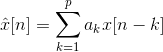
where x[n] is the predicted signal, p is the prediction order, and ak are the linear prediction coefficients [1].
There are three different ways to retrieve the linear prediction coefficients (ak, from equation 2.1): the auto-correlation method, the covariance method, and the Burg algorithm [3].
The difference between the signal x[n] and the predicted signal is known as the prediction error, which can be written as follows:
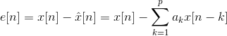
Therefore the prediction error is an FIR filter and its z-transform is:


Where P(z) in equation 2.3 is known as the Prediction filter [3]. The transfer function of equation 2.3 is:

Where A(z) is called the prediction error filter [3]. The inverse of the prediction error filter is called the synthesis filter or LPC filter [3] and is in the form:

The synthesis filter represents the spectral envelope (with a gain factor) of the input signal x[n] [3]. This means that if the prediction error is fed into the filter, you can recreate the input signal x[n] [3]. With a quantized prediction error signal, you can efficiently encode the input signal [3]. As well, the synthesis filter can be used to synthesize speech signals [4].

Chapter 3
Results
The following chapter presents some of the work involved in reproducing a selection of current research on the topic.
3.1 Initial Plots
Using the information in the DAFx book chapter by Arfib, Keiler, and Zölzer [3], an initial plot of the magnitude response of the synthesis filter was generated. The script was written in MATLAB to perform a similar analysis as the book chapter. The authors had written their own function to calculate the linear prediction coefficients, however, the code was modified to use the Matlab lpc function. A sound file of a female singer singing a solfège la note was found with the website freesound.org. The following figure shows the snippet of the signal used to calculate the prediction coefficents:
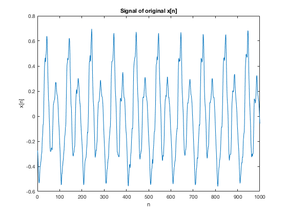 Figure 3.1: Input signal x[n]
Using a Hamming windowed version of the signal and a prediction order of 60, the spectra of the input signal and the synthesis filter were plotted on the same graph, as seen in the following figure:
 Figure 3.2: Plot of spectra for input signal and the synthesis filter
As was predicted, the spectrum of the synthesis filter closely follows the envelope of the input signal’s spectrum, with some additional gain. To see what effect the prediction order had on how closely the frequency spectrum follows the envelope of the input signal, another MATLAB script was written. The script calculates the prediction coefficients at 6 different prediction orders and plots them on the same graph. Additional offsets were added to each spectrum to provide some padding between the various plots. The resulting plot is shown in the following figure:
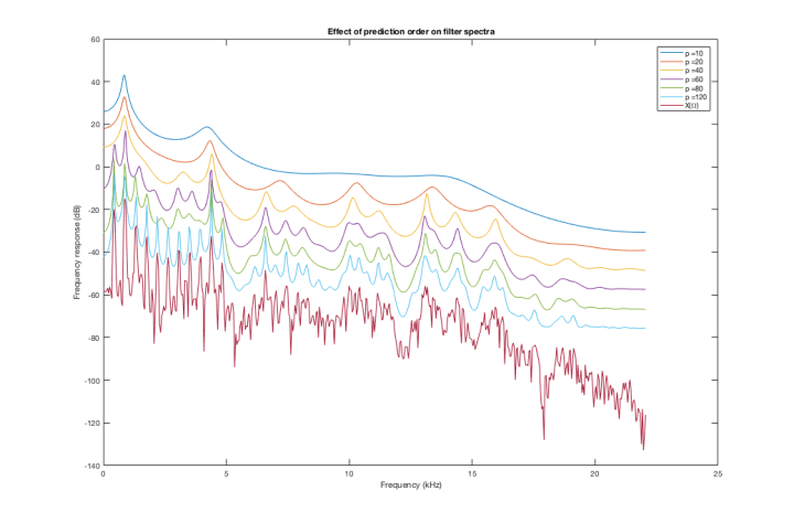
The figure presented similar results to what was shown in the paper. As the prediction order increased, the magnitude response of the synthesis filter follows the envelope of the input signal more closely.
3.2 Compensating for the gain
Reading the DAFx book chapter closer, it was determined that the authors had written their own function to calculate the prediction coefficients because they wanted to compensate for the gain offset that occurs. The MATLAB lpc function does not return the gain that inherently occurs when building the filter. However, the gain can easily be calculated when calculating the prediction coefficients [3].
Following the code presented in the paper more closely, a script was written that plots the two spectra that were seen in figure 3.2, but compensating for the additional gain in the synthesis filter. The following plot was generated in MATLAB:

As can be seen in the above figure, the spectrum of the synthesis filter is closer to the spectrum of the input signal and it is clear how closely it follows the input signal’s spectrum. As well, the book chapter plots the prediction error signal, because this can be used in computing the fundamental frequency of a sound [3]. The plot of the prediction error can be seen in the figure below:
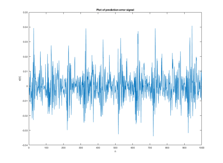 Figure 3.5: Plot of prediction error signal
As can be seen in the above figure, there are clear, periodic peaks in the prediction error signal. With this, the period of the fundamental frequency is 100 samples, which is 0.0023 seconds. At a sampling frequency of 44.1 kHz, this means the fundamental frequency of the original signal is 441 Hz.
3.3 LPC Speech Synthesis
As was shown in figure 2.1, speech synthesis is possible with an LPC synthesis filter [4]. To test this capability, a MATLAB script was written to attempt to re-synthesize the input waveform using only Gaussian white noise. The same input waveform was used with a much larger sample size and the prediction coefficients were calculated. Two seconds worth of samples of gaussian white noise were generated and passed through the filter pictured in figure 2.1. The resulting output waveform sounded similar to the input waveform, with some additional noise and effects.
Original Sound File:
Output Waveform:
A separate script was written to see what effect the prediction order had on the synthesized output waveform. Six separate audio files were generated, which attempts to synthesize the input waveform using prediction orders of 40, 60, 80, 120, 160, and 200. The original sound files and the generated sound files are included below:
- Original sound file:
- p = 40:
- p = 60:
- p = 80:
- p = 120:
- p = 160:
- p = 200:
Using a prediction order of less than 80, the resulting waveform sounded just like noise. At a prediction order of 80 and above the output waveform began to sound like the input, but with a large amount of reverberation. There were also diminishing returns in how much the sound quality increased with increasing the prediction order. Therefore, to be usable as a speech synthesizer, the prediction order needs to be chosen carefully.
Chapter 4
Discussion
The following chapter discusses the results obtained in chapter 3 and the experience of implementing the topic.
4.1 Discussion on Plots Generated
Using the information in the DAFx book chapter by Arfib, Keiler, and Zölzer [3], implementing an LPC synthesis filter was quite easy. Of course, the biggest difference between the implementation documented in section 3.1 and the implementation in the DAFx book chapter is the use of the MATLAB lpc function. The DAFx book chapter used their own custom function to calculate the prediction coefficients. A test was run to see if there was any difference between the two functions and found that both returned the same coefficients. So at first glance, it seemed unnecessary to use the custom function mentioned in the book chapter, and initial plots were generated using the MATLAB lpc function and similar results as the book chapter were generated.
However, upon closer inspection of the book chapter, it was found that this custom function was written because the authors wanted to retrieve the additional gain factor inherent in the implementation. The MATLAB lpc function returns only the coefficients and the variance of the prediction error. The first part of the book chapter however did not mention the gain in their first example, so it had seemed unnecessary. However in their next examples, it was quite useful to visualize how closely the synthesis filter response followed the input signal’s spectral envelope.
As well, at first glance the additional pre-samples that were pulled from the original signal and then subsequently removed seemed unnecessary. After running a test without them, it was seen that they were necessary to plot the prediction error in the same way as seen in the paper. Without the pre-samples, there were several samples of large prediction errors at the start of the plot. So the pre-samples shown in the book chapter were kept in the final code.
4.2 Discussion on LPC Speech Synthesis
Implementing the LPC speech synthesis was the most challenging aspect to this project. When first attempting to implement the block diagram shown in figure 2.1, it was not clear how the voiced/unvoiced switch shown worked. The first attempt at synthesizing speech based on the input signal’s prediction coefficients used a mixture of pulses and white noise, which did not generate good results. The next attempt used only pulses, which ended up generating some interesting percussive sounds, but not the recreation of the input signal that was predicted. Finally just the white noise was used, but the prediction order was too low and did generate a sound that was expected. Increasing the prediction order finally helped create a sound that was expected, but a lot of trial and error was used in order to create it.
Some future study in this would be to implement the model to work with full phrases like the paper by Atal and Hanauer showed results for [4]. This would be a good way to compare the implementation with the results in the paper.
Chapter 5
Conclusion
In conclusion, the theory behind LPC was presented and some applications of the tool based on research in the field was presented. An LPC synthesis filter was created with the research by Arfib, Keiler, and Zölzer [3]. This LPC synthesis filter was then used to create a rudimentary speech synthesizer using the research by Atal and Hanauer [4]. The results of this were analyzed and discussed. From this brief look at the topic, it is clear that LPC is a useful, multi-faceted tool with many applications.
Bibliography
[1] Wai C. Chu. Speech Coding Algorithms, chapter Linear Prediction, pages 91–142. John Wiley & Sons, Inc., 2004.
[2] J. Makhoul. Linear prediction: A tutorial review. Proceedings of the IEEE, 63(4):561–580, April 1975.
[3] D. Arfib, F. Keiler, and U. Zölzer. DAFx: Digital Audio Effects, chapter Source-filter Processing, pages 299–372. John Wiley & Sons, Ltd, 2004.
[4] B. S. Atal and Suzanne L. Hanauer. Speech analysis and synthesis by linear prediction of the speech wave. The Journal of the Acoustical Society of America, 50(2B):637–655, 1971.
